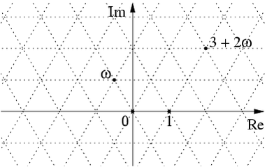
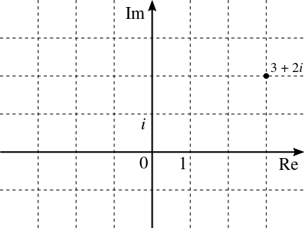
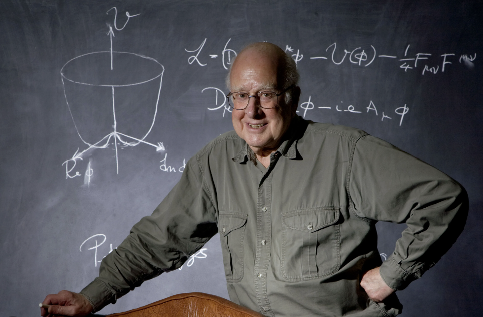
The Eisenstein integers are the complex numbers of the form where and are integers and . They form a subring of the complex numbers and also a lattice:
Last time I explained how the space of hermitian matrices is secretly 4-dimensional Minkowski spacetime, while the subset
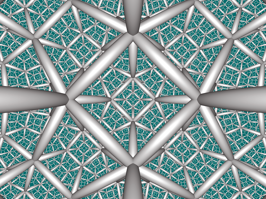
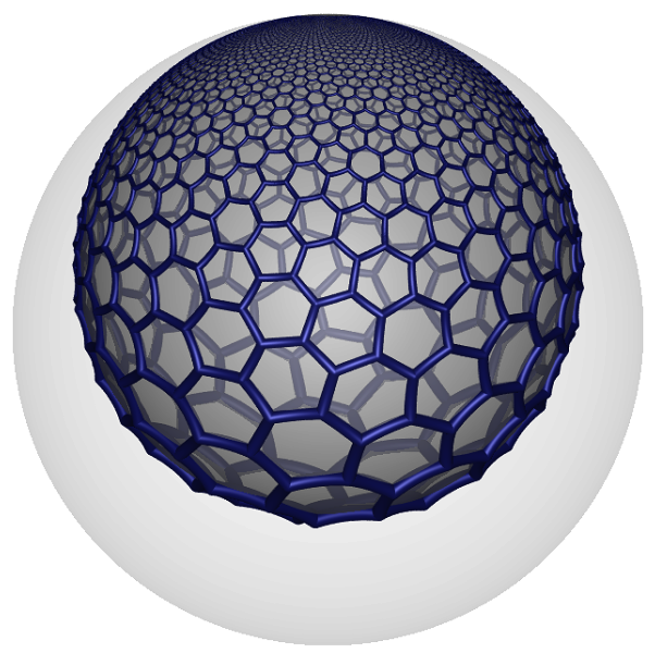
is 3-dimensional hyperbolic space. Thus, the set of hermitian matrices with Eisenstein integer entries forms a lattice in Minkowski spacetime, and I conjectured that consists exactly of the hexagon centers in the hexagonal tiling honeycomb — a highly symmetrical structure in hyperbolic space, discovered by Coxeter, which looks like this:
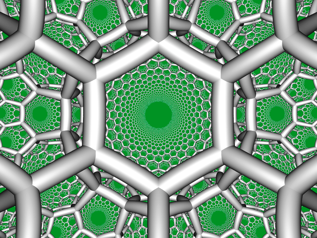
Now Greg Egan and I will prove that conjecture.
Last time, based on the work of Johnson and Weiss, we saw that the orientation-preserving symmetries of the hexagonal tiling honeycomb form the group . This is not only as an abstract isomorphism of groups: it’s an isomorphism of groups acting on hyperbolic space, where acts on and its subset by
and this action descends to the quotient .
By general abstract nonsense about Coxeter groups, the orientation-preserving symmetries of the hexagonal tiling honeycomb act transitively on the set of hexagon centers. Thus, if we choose a suitable point , we can get all the hexagon centers by acting on this one. Then the set of hexagon centers is this:
But what’s a suitable point ? I claim that the identity matrix will do, so
Once we show this, we can study the set in detail, allowing us to prove the result conjectured last time:
Theorem. , so the points in the lattice that lie on the hyperboloid are the centers of hexagons in a hexagonal tiling honeycomb.
But first things first: let’s see why the identity matrix can serve as a hexagon center!
The 12 hexagon centers closest to the identity
Suppose we take the identity as a hexagon center and get a bunch of points in hyperbolic space by acting on it by all possible transformations in . We get this set:
But how do we know this is right? We need to check that the points in this set look like the hexagon centers in here:
with the identity smack dab in the middle.
As you can see from the picture, each hexagon center should have 12 nearest neighbors. But does it work that way for our proposed set ? It will be enough to check that the identity matrix has 12 nearest neighbors in , and check that these 12 points are in . A symmetry argument then shows that each point in has 12 nearest neighbors arranged in the same pattern, so the points in are the centers of the hexagons in a hexagonal tiling honeycomb.
It’s easy to measure the distance to the identity matrix if you remember your hyperbolic trig. If we think of as Minkowski spacetime by writing a point as
then the time coordinate is . The distance in hyperbolic space from the identity to a point is then .
But this is a monotonic function of . So let’s find the points with the smallest possible trace — not counting the identity itself, which has trace . We hope there are 12.
Greg Egan found them:
(1)
and
(2)
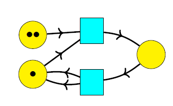
where and . These matrices are the 6 magenta points and 6 yellow points shown here, while the black point is the identity:
The dark blue points are hexagon vertices, which are not so important right now. By the way, the significance of is that it’s a primitive sixth root of unity; so is . So these give the hexagonal pattern we seek.
These 12 matrices clearly lie in , and they have determinant and positive trace so they lie in . But the good part is this:
Lemma 1. The 12 matrices in equations (1) and (2) are the matrices in that are as close as possible to the identity matrix without being equal to it. In other words, they have the smallest possible trace for matrices in .
I’ll put the proof of this and all the other lemmas in an appendix.
Now, why do these 12 matrices lie in
Greg found 12 matrices that do the job, namely
and
where .
A concrete construction of all the hexagon centers
Now we can get a concrete way to construct every element of the set
Lemma 2. The group consists of finite products of matrices of the form
for .
Lemma 3. Every element of is an element of multiplied on the right by some power of
Notice that this element is in but not in , and it acts on Minkowski space as a 60 degree rotation in the plane, giving the rotational symmetry in Greg’s image:
While we can implement this 60 degree rotation with an element of , namely
we cannot do it with any element of . This is why we need to bring into the game.
Lemma 4. The set equals the set of matrices where is a finite product of matrices of the form
for .
The theorem: first proof
Now we outline two proofs of the conjecture from last time. Greg did the hard part of the first proof, which uses some computer algebra we will only sketch. But the basic idea is this. We want to show that the points in the lattice that lie on the hyperboloid are precisely the centers of the hexagons in our hexagonal tiling honeycomb. It’s easy to show that all the hexagon centers lie in . The hard part is showing the converse. For this we assume we’ve got a point in that’s not a hexagon center. We assume it’s as close as possible to the identity matrix. Then, we’ll find another such point that’s even closer — so no such point could exist.
Theorem. The points in the lattice that lie on the hyperboloid are precisely the centers of hexagons in a hexagonal tiling honeycomb, since
Proof. Part of this theorem is easy. Unfolding the definitions, we need to show
But the only units in the Eisenstein integers are the 6th roots of unity, so for any its determinant is one of those, so and of course . This shows the set on the left-hand side is included in the set on the right-hand side.
So, the hard part is to show the reverse inclusion:
By Lemma 4, it suffices to assume has and , and prove that is of the form , where is a finite product of matrices
for or .
For a contradiction, suppose there exists with and that is not of this form. Since the set of such is discrete, we can choose one with the smallest possible trace. We now find one with a smaller trace, namely either or for some .
We can write
for integers obeying the extra conditions:
If we act on with each of the 12 elements , the changes in the trace of the original matrix are linear expressions in either and or and . It will only be impossible to reduce the trace if all 12 expressions are non-negative, for parameters where the determinant is 1.
It is easier to see what’s happening on a plot:

We would need to find values of and such that the green ellipse (the determinant condition) has a point with integer coordinates inside the smaller of the two hexagons (one of which scales with , the other with ).
The shape of the ellipse and hexagons are such that if the ellipse passed through any one hexagon vertex it would pass through all of them.
We can write the changes in the trace as:
Setting these to zero gives us the sides of the hexagons, while the vertices are found by solving:
to obtain:
The result for is the same, but with replaced by . Substituting these values into the formula for the determinant of and equating that to 1 gives us:
and for :
Without loss of generality we can assume , and use the curve defined by the second equation as the boundary for the region in the parameter space where the determinant ellipse contains points inside the -hexagon. The plot below shows that this only happens for , the identity matrix.
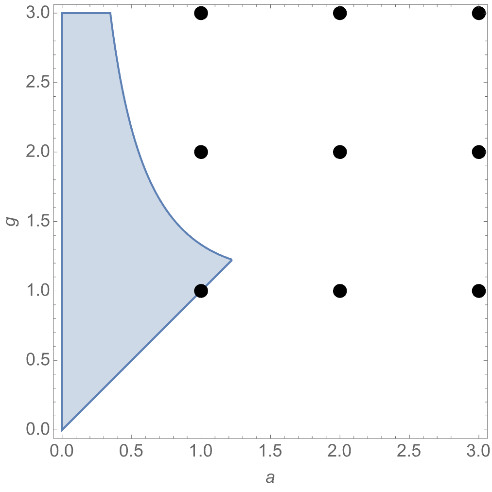
So, unless we are starting with the identity matrix, we can always act with one of the 12 elements and get an element with a smaller positive trace. █
The theorem: second proof
After Greg gave the above proof on Mathstodon, Mist gave a different proof which uses more about Coxeter groups. In this approach, the argument that keeps reducing the trace of a purported counterexample is replaced by the standard fact that every Coxeter group acts transitively on the chambers of its Coxeter complex. I will quote their proof word for word.
Theorem. The points in the lattice that lie on the hyperboloid are precisely the centers of hexagons in a hexagonal tiling honeycomb, since
Proof. Let me start with with elements denoted and equipped with the negative of the Minkowski form, that is, . Inside here, I choose vectors
By checking inner products, we see that these vectors and the aforementioned bilinear form determine a copy of the canonical representation of the rank-4 Coxeter group with diagram
where the 6 means that the edge is labeled ‘6’. My notation for the canonical representation is consistent with that of the Wikipedia article Coxeter complex.
By the general theory, the canonical representation acts transitively on the set of chambers, where the fundamental chamber is the tetrahedral cone cut out by the hyperplanes (through the origin) which are orthogonal to . Direct computation (e.g. matrix inverse) shows us that the extremal rays of the fundamental chamber are given by the vectors
Here I have dropped constant factors, but one can (and perhaps should) normalize to ensure Minkowski norm 1. Now I check explicitly that these vectors match up with Greg’s earlier explicit description of “a portion of the honeycomb”:
- The vector is one of the blue vertices of the hexagon centered on the black point.
- The vector after normalization becomes the midpoint of the two blue vertices indexed by and .
- The vector is the identity matrix, i.e. the black point.
- The vector (1, 0, 0, 1) is the null vector for one of the two horospheres which contains the hexagon centered on the black point.
According to the Wikipedia article Hexagonal tiling honeycomb, the desired honeycomb is constructed from the aforementioned Coxeter group by applying the Wythoff construction with only the first vertex circled. This confirms that the hexagon centers correspond to the vector and its images under the Coxeter group action.
It remains to show that the hexagon centers coincide with the elements of the Eisenstein lattice with Minkowski norm 1.
To show that the hexagon centers are contained in the Eisenstein lattice, it suffices to show that the Eisenstein lattice is invariant under the Coxeter group action. This follows by checking the action of each of the simple reflections:
In more detail, for , the inner product is a half-integer if is in the Eisenstein lattice, and the claim follows because is in the Eisenstein lattice. The same statement applies for and , and ‘half-integer’ can even replaced by ‘integer.’ For , the inner product is an integer multiple of , and the claim follows because is in the Eisenstein lattice.
To show that the elements of the Eisenstein lattice with Minkowski norm are hexagon centers, it suffices to show this statement within the fundamental chamber. Let be the null vector from before. Observe the following:
- If lies in the forward light cone, i.e. and , then .
- If lies in the Eisenstein lattice, then is an integer.
- If lies in the fundamental chamber and satisfies , then . (Sketch: Restricting to gives hyperbolic geometry, and the interior-of-horosphere is convex, so it suffices to check the special cases when is a vertex of the fundamental chamber.)
These observations imply that, if is an element of the Eisenstein lattice with lying in the fundamental chamber, then .
Next, write . Since rewrites as , the relation rewrites as . This tells us that the elements of the Eisenstein lattice with and are in bijection with the Eisenstein integers via
It is easy to check that the simple reflections preserve the aforementioned set of vectors and this bijection intertwines those simple reflections with the usual reflection symmetries of the Eisenstein integers (viewed as the vertices of the equilateral triangle lattice). Therefore, all of the aforementioned vectors v can be brought to via a Coxeter group action, as desired. █
What’s next?
A very similar theorem should be true for another regular hyperbolic honeycomb, the square tiling honeycomb:

Here instead of the Eisenstein integers we should use the Gaussian integers, , consisting of all complex numbers with .
Conjecture. The points in the lattice that lie on the hyperboloid are the centers of squares in a square tiling honeycomb.
I’m also very interested in how these results connect to algebraic geometry! That’s the real theme of this series, and I discussed the connection last time. Briefly, the hexagon centers in the hexagonal tiling honeycomb correspond to principal polarizations of the abelian variety . These are concepts that algebraic geometers know and love. Similarly, if the conjecture above is true, the square centers in the square tiling honeycomb will correspond to principal polarizations of the abelian variety . But I’m especially interested in interpreting the other features of these honeycombs — not just the hexagon and square centers — using ideas from algebraic geometry.
Proofs of lemmas
Lemma 1. The 12 matrices
are the points in that as close as possible to the identity matrix without being equal to it. In other words, they have the smallest possible trace for matrices in .
Proof. Matrices in are of the form
where , , the trace is and the determinant is . Since and are integers, and must be integers divided by 2.
The smallest possible trace for such a matrix is , realized only by the identity matrix. We are looking at the second smallest possible trace, which is . So, we have and , i.e. . Since is a half-integer and is an Eisenstein integer, the only options are to let and let be an Eisenstein integer of norm , i.e. a sixth root of unity. These give the matrices
for . █
Lemma 2. The group consists of finite products of matrices of the form
for .
Proof. In Section 8 of Quadratic integers and Coxeter groups, Johnson and Weiss cite Bianchi to say that is generated by these matrices:
The second and third of these matrices equal and , respectively, so we just need to write the first,
as a product of matrices and (or their inverses, which are again matrices of this form). Since
we have
Since the first matrix in this product is , it suffices to note that
is the product of and . █
Lemma 3. Every element of is an element of multiplied on the right by some power of
Proof. The determinant of any is some sixth root of unity, and the determinant of is a primitive sixth root of unity, so for some power we have
and thus . It follows that equals some element of , namely , multiplied on the left by some power of , namely . █
Lemma 4. The set equals the set of matrices where is a finite product of the matrices and .
Proof. By Lemma 3, is exactly the set of matrices where and
But the adjoint of is its inverse so
Thus, by Lemma 2, is exactly the set of matrices where is a finite product of the matrices and . █


 and
and  tell us how this common part fits into L and R.
 with:
with:

 in our collection, a timer
  This is a stochastic map
![T_i \colon [0,\infty) \to [0,\infty]](https://s0.wp.com/latex.php?latex=T_i+%5Ccolon+%5B0%2C%5Cinfty%29+%5Cto+%5B0%2C%5Cinfty%5D+&bg=ffffff&fg=333333&s=0&c=20201002)
 we get a probability measure
  on
on ![[0,\infty].](https://s0.wp.com/latex.php?latex=%5B0%2C%5Cinfty%5D.&bg=ffffff&fg=333333&s=0&c=20201002)
 to mean a randomly chosen element of
 ![[0,\infty]](https://s0.wp.com/latex.php?latex=%5B0%2C%5Cinfty%5D&bg=ffffff&fg=333333&s=0&c=20201002) distributed according to the probability measure
distributed according to the probability measure  We call
  we should wait until we apply the rewrite rule
  The time
 If you give me the initial state of the world
  the stochastic C-set rewriting system will tell you how to compute the state of the world at all later times. But this computation involves randomness.
 We look for all matches to patterns
  in the initial state
  For each match we compute a wait time
 ![w_i(t) \in [0,\infty]](https://s0.wp.com/latex.php?latex=w_i%28t%29+%5Cin+%5B0%2C%5Cinfty%5D&bg=ffffff&fg=333333&s=0&c=20201002) and then the rewrite time
and then the rewrite time  but right now
  is the first time the state of the world can change. We change it by applying the rewrite rule
  to the state of the world
  and its corresponding match from our table.
 we add that match and its rewrite time
  to our table.
 At that time, we apply the corresponding rewrite rule to the state
  , getting some new C-set
  We also cross off the rewrite time
  and its corresponding match from our table.
 here means the wait time can depend on when we start the timer. And the fact that this stochastic map takes values in
  However, in this case I am confused about how we should update our table of wait times as the state of the world changes. So I decided to postpone discussing this generalization!


 : they are
 equipped with the nondegenerate bilinear form
 with
with  and
and  But we can also think of Minkowski spacetime as the space
  of 2×2 hermitian matrices, using the fact that every such matrix is of the form


 are the complex numbers of the form
 and
and  are integers and
  is a cube root of 1. The Eisenstein integers are closed under addition, subtraction and multiplication, and they form a lattice in the complex numbers:
 of 2×2 hermitian matrices with Eisenstein integer entries gives a lattice in Minkowski spacetime, since we can describe Minkowski spacetime as
 are the centers of hexagons in a hexagonal tiling honeycomb.
 The hard part is showing that every point in
  is a hexagon center. Points in
  condition) and a quadratic equation (the
  condition). So, we’re trying to show that all 4-tuples obeying those constraints follow a very regular pattern.
 , consisting of all complex numbers
 that lie on the hyperboloid
  . These are concepts that algebraic geometers know and love. Similarly, if the conjecture above is true, the square centers in the square tiling honeycomb will correspond to principal polarizations of the abelian variety
  . But I’m especially interested in interpreting the other features of these honeycombs — not just the hexagon and square centers — using ideas from algebraic geometry.

.")


 , and a subset
  of
of  , we define the
 of
of  in
in  to be the set of all pairs
  where
where  are distinct elements of
 ![{[G:2G]}](https://s0.wp.com/latex.php?latex=%7B%5BG%3A2G%5D%7D&bg=ffffff&fg=000000&s=0&c=20201002) finite. Let
finite. Let  and
and  such that
  .
.  , but as noted in the recent preprint of
  has finite index. This condition is in fact necessary (as observed by forthcoming work of Ethan Acklesberg): if
  has infinite index, then one can find a subgroup
  of
of  for any
  that contains
  is
is  -torsion). If one lets
  be an enumeration of
 for any
  (indeed, from the pigeonhole principle and the
  one can show that
  must intersect
  whenever
  ). It is also necessary to work with restricted sums
  : a counterexample to the latter is provided for instance by the example with
  and
and ![{A := \bigcup_{j=1}^\infty [10^j, 1.1 \times 10^j]}](https://s0.wp.com/latex.php?latex=%7BA+%3A%3D+%5Cbigcup_%7Bj%3D1%7D%5E%5Cinfty+%5B10%5Ej%2C+1.1+%5Ctimes+10%5Ej%5D%7D&bg=ffffff&fg=000000&s=0&c=20201002) . Finally, the presence of the shift
. Finally, the presence of the shift  , though in the case
  one can of course delete the shift
  is a compact topological space (with the topology of pointwise convergence) (it is also metrizable since
  of
of  can be thought of as properties of subsets of
  that shares a sufficiently large (but finite) initial segment with
  elements.
  elements, where
  elements, where
  is the
  element of
  halts when given
  an
an  be a Følner sequence in
  , and let
  be a largeness property for each
  such that if
  is such that
  for all
  , then there exists a shift
  ,
,  ,
,  with
with  for all
  . By compactness, a subsequence of the
  . By openness, we conclude that there exists a finite
  . This implies that
  for infinitely many
  be as in Theorem
  between
  by declaring
  if
if  is an open subset of
 , then
  , and then any
  that contains both
  lies in
  .
.  of subsets of
  in
in  converges pointwise to
  and
and  converges pointwise to
  . (By
. (By  of
of  for all sufficiently large
  .)
.)
 and
and  be as in Theorem
  . Setting
  , we conclude that
  and
and  . Setting
  to be an even larger element of this sequence, we then have
  and
and  . Setting
  to be an even larger element, we have
  and
and  . Continuing in this fashion we obtain the desired infinite set
  to be a compact space
  equipped with a Borel probability measure
  as well as a measure-preserving homeomorphism
  . A point
  in
in  if one has
 . Define an (length three) dynamical Erdös progression to be a tuple
  in
in  and
and  .
.
 be a positive measure open subset of
  and
and  .
.  ,
,  , and
, and  for a Følner sequence
  with
with  , at which point Theorem
  of the Følner sequence are not required to contain the origin.)
 is a countable vector space over a finite field of size equal to an odd prime
  , so in particular
  ; we also specialize to Følner sequences of the form
  for some
  and
and  . In this case we can prove a stronger statement:
 for an odd prime
  be open subsets of
  . Then if
  , there exists an Erdös progression
  and
and  .
.  has full measure, so the hypothesis
  of Theorem
 ![{\mu(E_1)/[G:2G] + \mu(E_2) > 1}](https://s0.wp.com/latex.php?latex=%7B%5Cmu%28E_1%29%2F%5BG%3A2G%5D+%2B+%5Cmu%28E_2%29+%3E+1%7D&bg=ffffff&fg=000000&s=0&c=20201002) ; see Theorem 2.1 of
; see Theorem 2.1 of  be a compact metric space, let
  be a finite vector space over a field of odd prime order. Let
  , and let
  . Let
. Let  for some
  , there exist
  such that
 of open balls of radius
  . This induces a coloring function
  that assigns to each point in
  of the first ball
  that covers that point. This then induces a coloring
  of
of  . We also define the pullbacks
  for
for  . By hypothesis, we have
  , and it will now suffice by the triangle inequality to show that
 to be chosen later. This allows us to partition
  of index
  , such that on all but
 ![{\kappa [G:H]}](https://s0.wp.com/latex.php?latex=%7B%5Ckappa+%5BG%3AH%5D%7D&bg=ffffff&fg=000000&s=0&c=20201002) of these cosets
of these cosets  , all the color classes
  are
are  -regular in the Fourier (
 ) sense. Now we sample
  uniformly from
  ; as
; as  is also uniform in
  . By removing an exceptional event of probability
  , we may assume that neither of these cosetgs
  , we may also assume that
 . Similarly we may assume that


 -uniform in their respective cosets. Thus by standard Fourier calculations, we see that after excluding another exceptional event of probabitiy
 . By choosing
  small enough depending on
  , we can ensure that
  on
on  , we may assume that the
  grow as fast as we wish. Once we do so, we claim that for each
  , we can find
  such that for each
  , there exists
  that lies outside of
  such that
 converge to
  respectively, we obtain the desired Erdös progression.
 be a large parameter (much larger than
  converge vaguely to
  with
with  . Unfortunately,
  need not contain the origin.) However, we are assuming a continuous factor map
  to the Kronecker factor
  , which is a compact abelian group, and
  . As a consequence, we can find
  such that
  converges to
  converges to
  , so now
  converges vaguely to
  ,
,  , where
  is drawn uniformly at random from
  ,
,  ), but is easy to describe and will suffice for our argument. (A more appropriate choice, closer to the arguments of Kra et al., would be to
  , where the additional shift
  is a random variable in
  is a permutation on
  , and so

 denotes a quantity that goes to zero as
  (holding all other parameters fixed). By the hypothesis

 (compare with Theorem
  grow fast enough, we can then ensure that for each
  be the coloring function from the proof of Theorem
  ). Then it suffices to show that
 and
and  . This is a counting problem associated to the patterm
  ; if we concatenate the
  components of the pattern, this is a classic “complexity one” pattern, of the type that would be expected to be amenable to Fourier analysis (especially if one applies Cauchy-Schwarz to eliminate the
  ).
).
 of a level set of the coloring function
  is a bounded measurable function of
  that is measurable on the Kronecker factor, plus an error term
  that is orthogonal to that factor and thus is weakly mixing in the sense that
  tends to zero on average (or equivalently, that the Host-Kra seminorm
  vanishes). Meanwhile, for any
  , the Kronecker-measurable function
  , where
  is a bounded “trigonometric polynomial” (a finite sum of eigenfunctions) and
  . The polynomial
 , where
  is a bounded continuous function of
  norm at most
  , and
, and  is a bounded continuous function of
  (in practice we will take
  , we then have
 is just a sum of
  characters on
  such that these polynomial are constant on each coset of
  . Then
  and
and  . We then restrict
  to also lie in

 , which will establish our claim because
  .
.

 and
and  is annoying (as
  is an “infinite complexity” pattern that cannot be controlled by any uniformity norm), but (perhaps surprisingly) will not end up causing an essential difficulty to the argument, as we shall see when we start eliminating the terms in this sum one at a time starting from the right.
 term using
 , we may assume that the
  have normalized
  on both of these cosets
  . As such, the contribution of
  to
to  ). From the near weak mixing of the

 to
to  , if
, if  . Finally, the quantity
  is independent of
  in the coset
  . This density will be
  except for those
  which would have made a negligible impact on

 is small compared with
![{U^{s+1}[N]}](https://s0.wp.com/latex.php?latex=%7BU%5E%7Bs%2B1%7D%5BN%5D%7D&bg=ffffff&fg=000000&s=0&c=20201002) -norm
-norm filtration
![{[G_i,G_j] \leq G_{i+j}}](https://s0.wp.com/latex.php?latex=%7B%5BG_i%2CG_j%5D+%5Cleq+G_%7Bi%2Bj%7D%7D&bg=ffffff&fg=000000&s=0&c=20201002) for all
for all  . The weaker notion (sometimes known as a prefiltration) permits the group
  to be strictly smaller than
  , while the stronger notion requires
  was a central group, which is true for filtrations, but not necessarily for prefiltrations. This fact (or more precisely, a multidegree variant of it) was used to claim a factorization for a certain product of nilcharacters, which is in fact not true as stated. In the erratum, a substitute factorization for a slightly different product of nilcharacters is provided, which is still sufficient to conclude the main result of this part of the paper (namely, a statistical linearization of a certain family of nilcharacters in the shift parameter
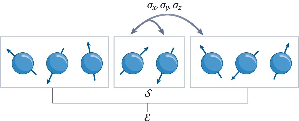
 of states,
 of transitions,
 mapping each transition to its upstream and downstream states.
 is the disjoint union of
  We get four cases:
 of agents. To handle births and deaths, I wanted to make this set time-dependent. But I need to separately say how this works for transformations, birth transitions and death transitions. For transformations we don’t change
  For birth transitions we add a new element to
  and maybe record its name on a ledger or drive a stake through its heart to make sure it can never be born again!
 and the agents at states linked to the transition
  form some set
  when will agent
  , they don’t have a time at which they arrived at that state.
 in an unborn state. This can be done without using an infinite amount of memory: it’s a ‘potential infinity’ rather than an ‘actual infinity’.
 of vertices or states,
 of edges or transitions,
 mapping each edge to its source and target, also called its upstream and downstream,
 of links,
 and
and  mapping each link to its source (a state) and its target (a transition).
 will undergo a transition
  if it arrives at the state upstream to that transition at a specific time
  This jump function will not be deterministic: it will be a stochastic function, just as it was in
  and
and  But now the links will come into play.
 will have one state
  as its source. We say this state affects the transition
 So, we want the jump function for the transition
 And as mentioned earlier, the jump function will also depend on a choice of agent
 for each transition
 is the answer to this question:
 and the agents at states linked to the edge
  given that it doesn’t do anything else first?
 can keep changing. This is the big difference between today’s formalism and yesterday’s.
 namely:

 when will agent
 an agent makes a transition. More specifically, suppose agent
  makes a transition
  from the state


 (by removing
  from this subset) and in the state
  (by adding
  that’s affected by the state
 is the element of
  saying which subset of agents is in each state affecting the transition
  (So, we update our table of times at which agent
  given that it doesn’t do anything else first.)
 And we need to compute what actually happens then!
 for each agent
 replacing


 ︎
︎


 for all
  ), and let
  . Then
  translates of a subgroup
  . Moreover,
  for some
  .
. case of this result, with the number of translates bounded by
  (which was subsequently improved to
  by Jyun-Jie Liao), but without the additional containment
  . It remains a challenge to replace
  by a bounded constant (such as
  be independent finitely supported random variables on
 ![\displaystyle {\bf H}[X_1+\dots+X_m] - \frac{1}{m} \sum_{i=1}^m {\bf H}[X_i] \leq \log K,](https://s0.wp.com/latex.php?latex=%5Cdisplaystyle+%7B%5Cbf+H%7D%5BX_1%2B%5Cdots%2BX_m%5D+-+%5Cfrac%7B1%7D%7Bm%7D+%5Csum_%7Bi%3D1%7D%5Em+%7B%5Cbf+H%7D%5BX_i%5D+%5Cleq+%5Clog+K%2C&bg=ffffff&fg=000000&s=0&c=20201002)
 denotes Shannon entropy. Then there is a uniform random variable
  on a subgroup
 ![\displaystyle \frac{1}{m} \sum_{i=1}^m d[X_i; U_H] \ll m^3 \log K,](https://s0.wp.com/latex.php?latex=%5Cdisplaystyle+%5Cfrac%7B1%7D%7Bm%7D+%5Csum_%7Bi%3D1%7D%5Em+d%5BX_i%3B+U_H%5D+%5Cll+m%5E3+%5Clog+K%2C&bg=ffffff&fg=000000&s=0&c=20201002)
 take values in some symmetric set
  , then
  for some
  .
. of
of ![\displaystyle {\bf H}[X_1+\dots+X_m] - \frac{1}{m} \sum_{i=1}^m {\bf H}[X_i]](https://s0.wp.com/latex.php?latex=%5Cdisplaystyle+%7B%5Cbf+H%7D%5BX_1%2B%5Cdots%2BX_m%5D+-+%5Cfrac%7B1%7D%7Bm%7D+%5Csum_%7Bi%3D1%7D%5Em+%7B%5Cbf+H%7D%5BX_i%5D+&bg=ffffff&fg=000000&s=0&c=20201002)
 , but as we are not attempting to completely optimize the constants, we did not do so in the current paper (and as such, our arguments here give a slightly different way of establishing the
  random variables
  for
for  , with each
  of our array will end up being close to independent of the column sums
  , subject to conditioning on the total sum
  . Not coincidentally, this type of conditional independence phenomenon also shows up when considering row and column sums of iid independent gaussian random variables, as a specific feature of the gaussian distribution. It is related to the more familiar observation that if
  are two independent copies of a Gaussian random variable, then
  and
and  are also independent of each other.
 array of random variables as opposed to some other shape of array. But now the torsion enters in a key role, via the obvious identity
 ($1.048 million) has been allocated for various prizes associated to this competition. More detailed rules can be found
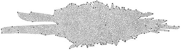


